Topic 22

Image enhancement is a very basic image processing task that defines us to have a better subjective judgement over the images. And Image Enhancement in spatial domain (that is, performing operations directly on pixel values) is the very simplistic approach. Enhanced images provide better contrast of the details that images contain. Image enhancement is applied in every field where images are ought to be understood and analysed. For example, Medical Image Analysis, Analysis of images from satellites, etc. Here I discuss some preliminary image enhancement techniques that are applicable for grey scale images.

Image enhancement simply means, transforming an image f into image g using T. Where T is the transformation. The values of pixels in images f and g are denoted by r and s, respectively. As said, the pixel values r and s are related by the expression,

where T is a transformation that maps a pixel value r into a pixel value s. The results of this transformation are mapped into the grey sclale range as we are dealing here only with grey scale digital images. So, the results are mapped back into the range [0, L-1], where L=2^k, k being the number of bits in the image being considered. So, for instance, for an 8-bit image the range of pixel values will be [0, 255].

There are three basic types of functions (transformations) that are used frequently in image enhancement. They are,

• Linear,
• Logarithmic,
• Power-Law.

The transformation map plot shown below depicts various curves that fall into the above three types of enhancement techniques.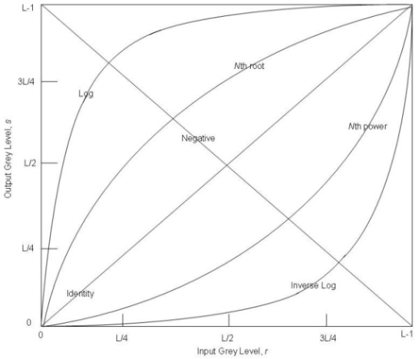

Figure A: Plot of various transformation functions

The Identity and Negative curves fall under the category of linear functions. Indentity curve simply indicates that input image is equal to the output image. The Log and Inverse-Log curves fall under the category of Logarithmic functions and nth root and nth power transformations fall under the category of Power-Law functions.

The negative of an image with grey levels in the range [0, L-1] is obtained by the negative transformation shown in figure above, which is given by the expression,

This expression results in reversing of the grey level intensities of the image thereby producing a negative like image. The ouput of this function can be directly mapped into the grey scale look-up table consisting values from 0 to L-1.

The log transformation curve shown in fig. A, is given by the expression,

where c is a constant and it is assumed that r≥0. The shape of the log curve in fig. A tells that this transformation maps a narrow range of low-level grey scale intensities into a wider range of output values. And similarly maps the wide range of high-level grey scale intensities into a narrow range of high level output values. The opposite of this applies for inverse-log transform. This transform is used to expand values of dark pixels and compress values of bright pixels.

The nth power and nth root curves shown in fig. A can be given by the expression,

This transformation function is also called as gamma correction. For various values of γ different levels of enhancements can be obtained. This technique is quite commonly called as Gamma Correction. If you notice, different display monitors display images at different intensities and clarity. That means, every monitor has built-in gamma correction in it with certain gamma ranges and so a good monitor automatically corrects all the images displayed on it for the best contrast to give user the best experience.

The difference between the log-transformation function and the power-law functions is that using the power-law function a family of possible transformation curves can be obtained just by varying the λ.

These are the three basic image enhancement functions for grey scale images that can be applied easily for any type of image for better contrast and highlighting. Using the image negation formula given above, it is not necessary for the results to be mapped into the grey scale range [0, L-1]. Output of L-1-r automatically falls in the range of [0, L-1]. But for the Log and Power-Law transformations resulting values are often quite distintive, depending upon control parameters like λ and logarithmic scales. So the results of these values should be mapped back to the grey scale range to get a meaningful output image. For example, Log function s = c log(1 + r) results in 0 and 2.41 for r varying between 0 and 255, keeping c=1. So, the range [0, 2.41] should be mapped to [0, L-1] for getting a meaningful image.

Reference:
Gonzalez C. R., Woods E. R., Digital Image Processing, 2nd Ed., 2000. Prentice Hall, New Jersey.

By the way, just as a note, spellings Grey and Gray mean one and the same.

V Rama Aravind,
2006-03-01.
Posted on: 2006-03-02.